
More Information
Submitted: February 12, 2026 | Accepted: February 19, 2026 | Published: February 20, 2026
Citation: Sridhar LN. Analysis and Control of the Hodgkin-Huxley Model. Arch Psychiatr Ment Health. 2026; 10(1): 006-013. Available from:
https://dx.doi.org/10.29328/journal.apmh.1001061
DOI: 10.29328/journal.apmh.1001061
Copyright license: © 2026 Sridhar LN. This is an open access article distributed under the Creative Commons Attribution License, which permits unrestricted use, distribution, and reproduction in any medium, provided the original work is properly cited.
Keywords: Bifurcation; Optimization; Control; Neuron; Hopf

Analysis and Control of the Hodgkin-Huxley Model
Lakshmi N Sridhar*
Chemical Engineering Department, University of Puerto Rico, Mayaguez, PR 00681, USA
*Corresponding author: Lakshmi N Sridhar, Chemical Engineering Department, University of Puerto Rico, Mayaguez, PR 00681, USA, Email: [email protected]
Objective: The Hodgkin-Huxley model is one of the most influential mathematical models in neuroscience, describing how electrical activity is generated and propagated in neurons. In this work, bifurcation analysis and Multiobjective Nonlinear Model Predictive Control are performed on the dynamic Hodgkin-Huxley model.
Methods: The MATLAB program MATCONT was used to perform the bifurcation analysis. The MNLMPC calculations were performed using the optimization language PYOMO in conjunction with the state-of-the-art global optimization solvers IPOPT and BARON.
Results: The bifurcation analysis revealed the existence of Hopf bifurcation points and limit points. The MNLMC converged on the Utopian solution. Hopf bifurcation points, which cause unwanted limit cycles, are eliminated using an activation function based on the tanh function.
Conclusion: The limit points (which cause multiple steady-state solutions from a singular point) are very beneficial because they enable the Multiobjective Nonlinear Model Predictive Control calculations to converge to the Utopia point (the best possible solution) in the model. The tanh activation function is highly effective at eliminating Hopf Bifurcations.
The Hodgkin-Huxley model was developed by Alan Hodgkin and Andrew Huxley in 1952, following their groundbreaking experiments on the squid giant axon, in which they described how an action potential is generated by the combined effects of ion currents across the neuronal membrane. The development of this mathematical model was revolutionary in the biological sciences, as it showed that complex biological processes can be described by coupled nonlinear equations.
The heart of the Hodgkin-Huxley model is the modelling of the neuronal membrane as an electric circuit. The neuronal membrane has a lipid bilayer that functions as a capacitor, storing charge. Additionally, membrane ion channels function as dynamic ion conductances, allowing certain ions to pass. The model primarily discusses sodium (Na⁻) and potassium (K⁻) ions, with a leakage current representing the other ions. The movement of ions along electrochemical gradients determines changes in neuronal membrane potential. The key innovation of this model is its incorporation of ion-channel dynamics via gating variables. Instead of having channels either open or shut, Hodgkin and Huxley proposed using probabilistic variables that reflect how many of the channel gates are in an open state. For sodium channels, there are two gating components: activation and inactivation; by contrast, only activation gating is present in potassium channels. The dynamics of these gating variables are governed by voltage-dependent rate equations. In this way, the model reproduced the upstroke, peak, and repolarization phases of an action potential with high accuracy.
The non-linear aspect of the Hodgkin-Huxley equations has been found to underpin their explanatory power. A small perturbation in membrane potential might be dampened, but once the critical threshold is breached, the positive feedback from sodium channels enables rapid depolarization. This all-or-nothing response accounts for the characteristic action potential as well as the maintenance of the same strength as it propagates down the length of the axon. The delayed opening of potassium channels and the closure of sodium channels enable the refractory phase.
Beyond analyzing single action potentials, the Hodgkin-Huxley model can be used to study repetitive firing, frequency modulation, and neuronal responses to external stimuli. This can be achieved by varying certain parameters, such as ion conductances and current, to demonstrate different dynamic properties, including steady states, regular spiking, and complex transients. This has placed the Hodgkin-Huxley model at the heart of neuronal excitation studies and of other ideas such as threshold behavior, relaxation, and bifurcations in biological systems.
Although highly successful, the Hodgkin-Huxley model is not without limitations. It is numerically intensive because it is a system of several coupled equations, which can be cumbersome during computational modelling of large neuronal networks. However, unlike more complex models, it approximates the behavior of ion channels and does not address stochastic processes or the microscopic nature of these channels. Many reduced neuron models, including the FitzHugh-Nagumo and integrate-and-fire models, derive from the original Hodgkin-Huxley neuron model.
The Hodgkin-Huxley model remains a landmark accomplishment in mathematical biology and neuroscience as it combined experimental findings and mathematical formulation to expose the mechanisms of neuronal excitation. The implications of this theory certainly lie within its own realm of application, where it remains at the forefront of neuroscience and mathematical modelling of nonlinear dynamics in living systems.
The Hodgkin-Huxley model is an iconic nonlinear dynamic system that models the electrical activity of excitable nerve cell membranes. The HH model comprises four coupled ordinary differential equations that describe the membrane potential and the gating variables of the sodium and potassium channels in the cell membrane. The HH model possesses rich dynamic behavior on its own because it inherently has feedback and nonlinearities. These inherently create limit cycles in the HH model.
Limit cycles of the Hodgkin-Huxley equations correspond to the existence of a stable self-sustained oscillation of the membrane potential. Physiologically, oscillations correspond to the repetitive firing of action potentials, which is an important component of neuronal activity. The Hodgkin-Huxley equations correspond to stable equilibrium points of the resting membrane potential at low applied current. When the applied current exceeds the threshold level, the system reaches an unstable equilibrium point, and as a result, it enters a limit cycle of oscillations, corresponding to the periodic solution of the equations.
Typically, the Hopf bifurcation is the most common mechanism for the emergence of limit cycles in the HH model. Above a certain critical level of the injected current, the pair of complex-conjugate eigenvalues of the linearization of the system crosses the imaginary axis, causing instability of the steady-state solution and leading to the birth of a small limit cycle that can further develop into a large limit cycle representing spiking activity. Depending on the choice of parameter values, the Hopf bifurcation can be either subcritical or supercritical.
Limit cycles of the HH model are more than mathematical concepts and play crucial roles in biologically essential processes. Limit cycles facilitate the transition from quiescence to rhythmic firing and provide insights into other rhythmic activities, such as frequency-current curves and neuronal excitability types. Pathological limit cycle activities also relate to the inappropriate rhythmic activities of the brain, for instance, seizure activities that occur during epileptic seizures.
The existence of limit cycles in the Hodgkin-Huxley equations stems from nonlinear ion-channel dynamics and bifurcation theory. Limit cycles provide valuable models of neuronal repetitive firing and mechanisms of neuronal excitability from a dynamical perspective.
Limit cycles in the Hodgkin-Huxley (HH) model correspond to self-sustained oscillations of the membrane potential, which lead to repetitive firing of action potentials. The phenomenon of limit-cycle oscillations has physiological implications and may be expressed by neurons under various conditions. However, self-sustained limit cycles in the HH model could be undesirable when modelling the physiological functioning of the cell, as actual neuronal excitation in living organisms, as a rule, follows the external excitation of the cell and is followed by a recovery phase to the resting state, which corresponds to a stable limit cycle. From a physiological point of view, a persistent oscillatory firing is energetically expensive. This is because the cycling of sodium and potassium ions requires continuous operation of ion pumps to maintain the ion gradient. This is not only at variance with the energy-efficient mode of operation of most neurons but is only currently observable under pathological conditions. From a functional perspective, limit cycles in the HH model are undesirable. Indeed, the persistent oscillations reduce a neuron’s ability to encode information into stimulus-dependent firing patterns because the system dynamics become dominated by the intrinsic oscillations rather than by the external signals. In networks, this can lead to excessive synchronization or runaway activity. For these reasons, the stable equilibria with stimulus-dependent spiking are generally preferred over autonomous limit cycles when modelling normal neuronal excitability and responsiveness.
One of the main aims of this paper is to demonstrate a computational strategy that can effectively eliminate the Hopf bifurcations that give rise to limit cycles.
The Hodgkin–Huxley model [1] presents a quantitative description of membrane current and its application to conduction and excitation in nerve. Fitzhugh [2] discussed several mathematical models of excitation and propagation in the nerve. Chay and Keizer [3] developed a minimal model of membrane oscillations in the pancreatic 𝛽-cell. Bedrov, et al. [4] investigated the partition of the Hodgkin-Huxley-type model parameter space into regions of qualitatively different solutions. Guckenheimer and Labouriau [5] performed a unique bifurcation analysis of the Hodgkin and Huxley equations.
Bedrovv, et al. [6] developed a method for constructing the boundary of the bursting oscillation region in a neuron model. Fukai and co-workers, [7,8] discussed Hopf bifurcations in the multiple-parameter space of the Hodgkin-Huxley equations. Zhu, et al. [9] discussed the equilibrium point bifurcation and the singularity analysis of the HH Model with Constraint.
In this work, bifurcation analysis and multiobjective nonlinear model predictive control are performed for the Hodgkin–Huxley model Zhu, et al. [9]. The paper is organized as follows. First, the model equations are presented, followed by a discussion of the numerical techniques involving bifurcation analysis and multiobjective nonlinear model predictive control (MNLMPC). The results and discussion are then presented, followed by the conclusions.
Model equations
In the model equations, vv represents the membrane potential. The variables mv and hv are the gating variables representing activation and inactivation of the Na+ current, while NV is the gating variable representing activation of the K+ current. IV represents the external current. represent the K+, Na+, and leak currents. 𝑔Na and 𝑔K,
representing the maximal conductance of sodium and potassium. cm represents the membrane capacitance.
The model equations are:
(1)
Where
The base parameter values are
Bifurcation analysis
Bifurcation analysis is done with MATCONT [10,11], a commonly used MATLAB program that locates limit points, branch points, and Hopf bifurcation points. This program detects Limit points (LP), branch points (BP), and Hopf bifurcation points (H) for an ODE system.
(2)
Let the bifurcation parameter be. Since the gradient is orthogonal to the tangent vector,
The tangent plane at any point must satisfy.
(3)
Where A is
(4)
Where is the Jacobian matrix? At the limit and branch points, the Jacobian matrix must be singular.
For a limit point, the n+1Th component of the tangent vector = 0, and at a branch point (BP), the matrix must be singular.
For a Hopf bifurcation,
(5)
@ indicates the bilateral product, while In is the n-square identity matrix. Hopf bifurcations cause limit cycles and should be eliminated because limit cycles make optimization and control tasks very difficult. More details can be found in [12-14].
Hopf bifurcations cause limit cycles. The tanh activation function (where a control value u is replaced by) is used in control problems [15-19] used the activation factor involving the tanh function to eliminate Hopf bifurcation points.
Multiobjective Nonlinear Model Predictive Control (MNLMPC)
The strategy for the multiobjective nonlinear model predictive control (MNLMPC) is similar to that of Flores Tlacuahuaz, et al. [20].
In a situation where the variables (j=1, 2...n) have to be optimized simultaneously for a dynamic problem
(6)
being the final time value, and n the total number of objective variables, u the control parameter. The single objective optimal control problem is solved independently optimizing each of the variables the optimization of will lead to the values . Then, the multiobjective optimal control (MOOC) problem that will be solved is
(7)
This will provide the values of u at various times. The first obtained control value of u is implemented, and the rest are discarded. This procedure is repeated until the implemented and the first obtained control values are the same, or until the Utopia point, where ( for all j) is obtained.
Pyomo [21] is used for these calculations in conjunction with IPOPT [22] and BARON [23].
Sridhar [24] demonstrated that the presence of limit and branch points enabled the MNLMPC calculations to converge to the Utopia solution. This was done by imposing the singularity condition, caused by the presence of the limit or branch points, on the co-state equation [25]. These numerical procedures are very similar to those used in Sridhar [26].
Bifurcation analysis is performed with several bifurcation parameters. In each of the cases, the use of an activation factor involving the tanh function removes the unwanted limit cycle causing Hopf bifurcations, validating the hypothesis of Sridhar [21].
When iv is the bifurcation parameter, 2 Hopf bifurcation points and 2 limit points were found at values of (4.315738, 0.086823, 0.442071, 0.385365, -9.406583); (35.263043, 0.739314, 0.01874, 0.773422, -13.971904); (5.583270, 0.099806, 0.398118, 0.405571, -9.261244 ); and (25.615543, 0.516846, 0.047253, 0.685295, -38.368717). This is shown in curve AB in Figure 1a. When iv is changed to (iv ((tanh (iv)/-4) the Hopf bifurcations disappear, and a limit point occurs at (5.583312 0.099807 0.398116 0.405572 37.044974). This is seen in curve CD in Figure 1a. The limit cycles for these two Hopf bifurcation points are shown in Figure 1b and Figure 1c.
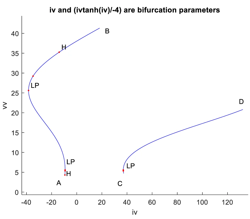
Figure 1a: Hopf bifurcation occurs when IV is the bifurcation parameter (AB) and disappears when IV is modified to ivtanh (IV)/-4.
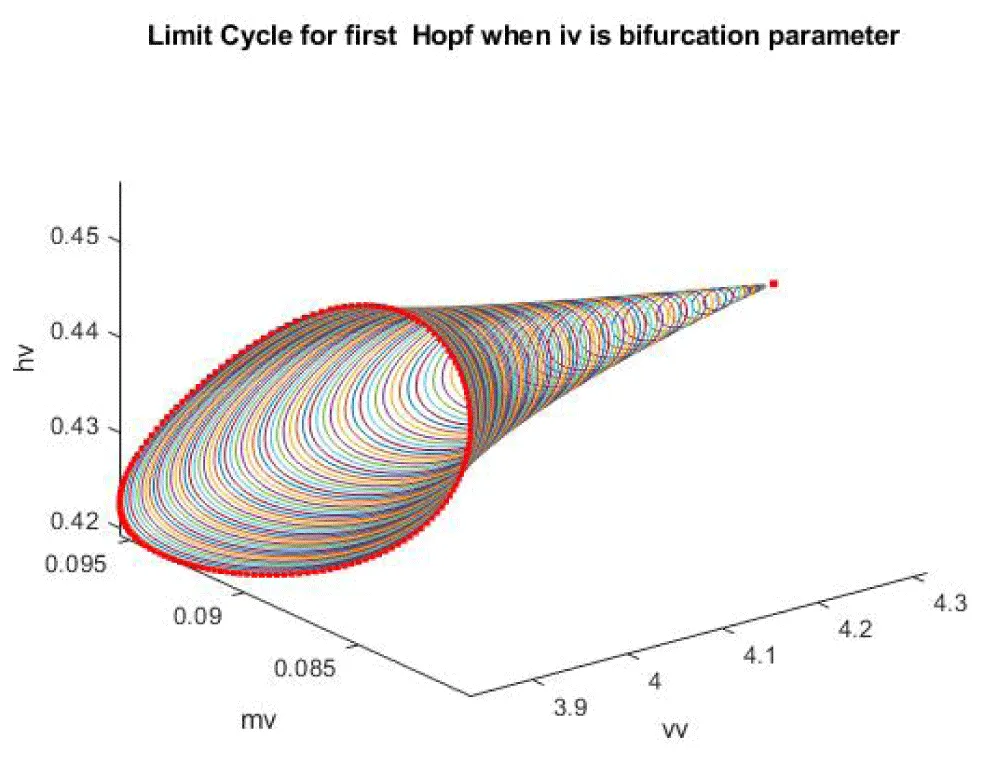
Figure 1b: Limit Cycle for first Hopf when IV is the bifurcation parameter.
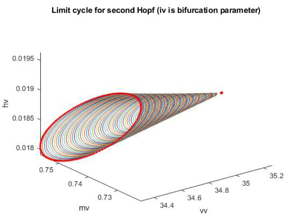
Figure 1c: Limit Cycle for the second Hopf when IV is the bifurcation parameter.
When gk is the bifurcation parameter, 2 Hopf bifurcation points were found at values of (8.916507, 0.141771, 0.292738, 0.458508, 34.941511); (33.004623, 0.694442, 0.022858, 0.755492, 4.973283). This is shown in curve AB in Figure 2a. When IV is changed to (gk ((tanh (IV)/2.1) the Hopf bifurcations disappear. This is seen in curve CD in Figure 2a. The limit cycles for these two Hopf bifurcation points are shown in Figure 2b and Figure 2c.
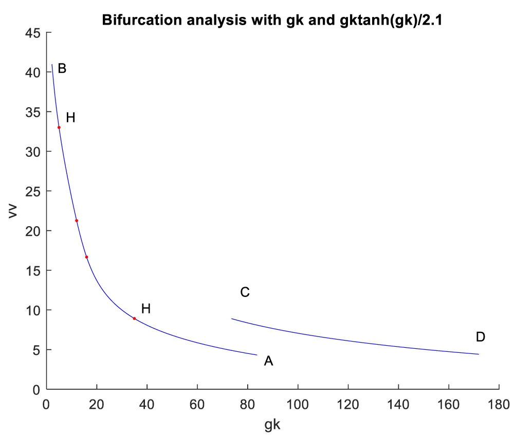
Figure 2a: Hopf bifurcation occurs when gk is the bifurcation parameter (AB) and disappears when IV is modified to gktanh (gk)/2.1.
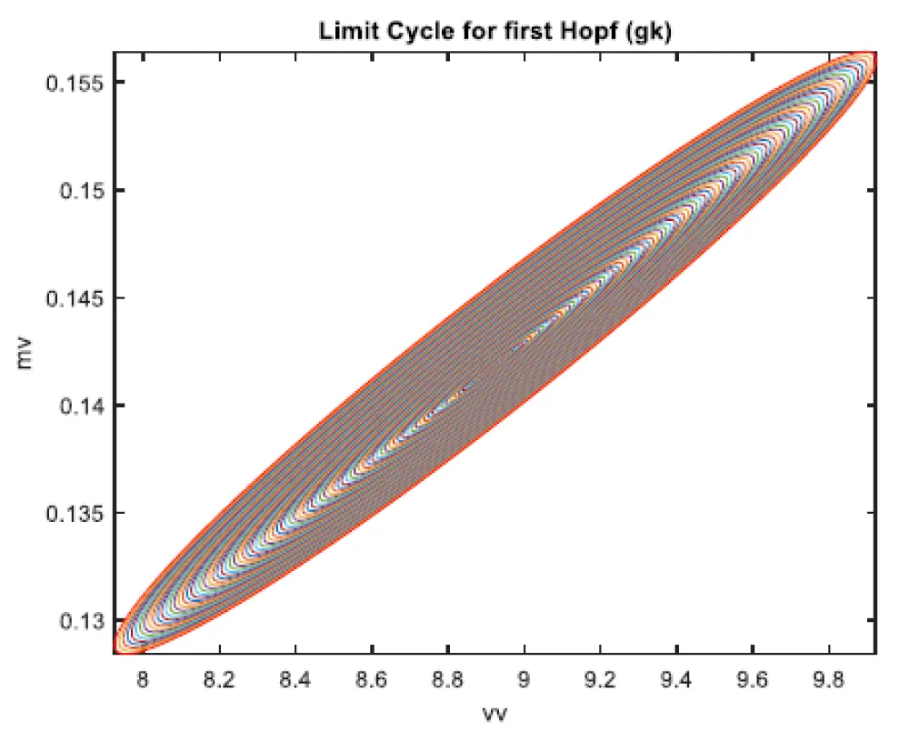
Figure 2b: Limit Cycle for first Hopf (gk is bifurcation parameter).
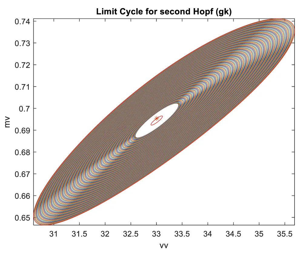
Figure 2c: Limit Cycle for second Hopf (gk is the bifurcation parameter).
When vk is the bifurcation parameter, a Hopf bifurcation points were found at values of (4.819640, 0.091802, 0.424415, 0.393393, and 624.006805). This is shown in curve AB in Figure 3a. When IV is changed to (vk ((tanh (vk)/-3), the Hopf bifurcation disappears. This is seen in curve CD in Figure 3a. The limit cycle for this Hopf bifurcation point is shown in Figure 3b.
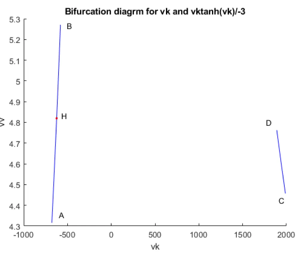
Figure 3a: Hopf bifurcation occurs when vk is the bifurcation parameter (AB) and disappears when vk is modified to vktanh (vk)/-3.
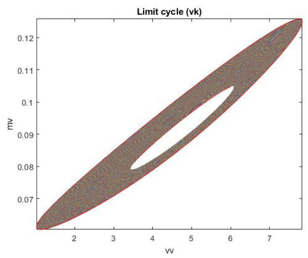
Figure 3b: Limit Cycle for Hopf (vk is the bifurcation parameter).
When vl is the bifurcation parameter, 2 Hopf bifurcation points and 2 limit points were found at values of (4.315738, 0.086823, 0.442071, 0.385365, -18.807583); (35.263043, 0.739314, 0.01874, 0.773422, -23.372904); (5.58327, 0.099806, 0.398118, 0.405571, -18.662244); (25.615543, 0.516846, 0.047253, 0.685295, -47.769717). This is shown in curve AB in Figure 4a. When vl is changed to (vl((tanh(vl)/-3) the Hopf bifurcation disappears, but two limit points occur at (5.583312, 0.099807, 0.398116, 0.405572, 55.986731);(25.615553, 0.516847, 0.047253, 0.685295, 143.309151). This is seen in curve CD in Figure 4a. The limit cycles for the two Hopf bifurcation points are shown in Figures 4b and 4c.
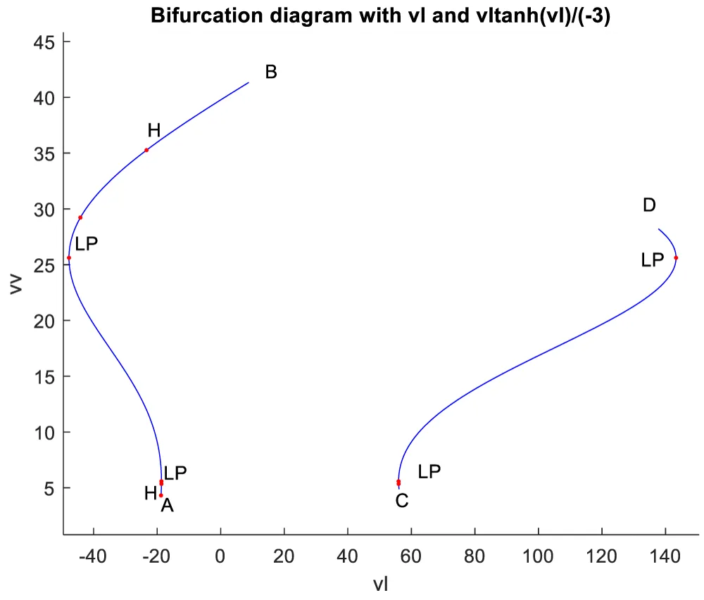
Figure 4a: Hopf bifurcation occurs when vl is the bifurcation parameter (AB) and disappears when vl is modified to vltanh(vl)/-3.
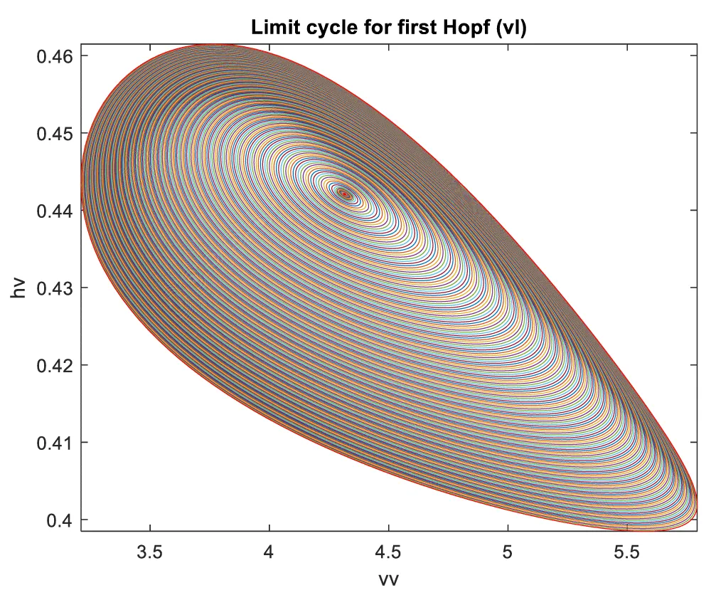
Figure 4b: Limit Cycle for first Hopf (vl is bifurcation parameter).
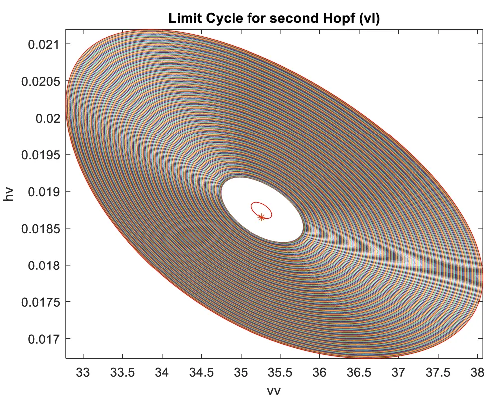
Figure 4c: Limit Cycle for second Hopf (vl is bifurcation parameter).
In all cases, the use of the tanh activation function eliminates the Hopf bifurcation point, thereby validating the analysis of Sridhar [19]. In this regard, the elimination of Hopf bifurcations in the Hodgkin-Huxley model is usually an issue of interest when one wants to ensure that the neuronal behavior is stable and predictable, without pathological or non-physiological oscillations. A Hopf bifurcation means the transition of an equilibrium from being stable to unstable, which gives rise to sustained oscillations and limit cycles in the membrane potential. This type of transition bears significant physiological and modelling implications within neuronal dynamics.
Hopf bifurcations are associated with the onset of repetitive firing. Though oscillatory spiking is a normal feature in neurons under specific stimuli, uncontrolled or unintended oscillations in the HH model represent abnormal neural activity. These dynamics are very often related to pathological conditions such as epilepsy, tremors, and neuropathic pain, where neurons may fire excessively or in a self-sustained way. Elimination of Hopf bifurcations helps prevent these regimes and guarantees that neurons will return to a stable resting potential in the absence of appropriate external inputs. In this context, the removal of Hopf bifurcations in the Hodgkin-Huxley model is typically a concern when one seeks to guarantee stability and predictability of neuronal dynamics. When a Hopf bifurcation occurs, it signifies the instability of an equilibrium state, which becomes an unstable state that produces oscillations of the limit-cycle type in the neuronal membrane potential. Hopf bifurcations are commonly related to periodic firing. Although oscillatory spiking is a normal phenomenon in certain stimuli for a neuron, any form of uncontrolled, unintended oscillations in an HH neuron model denotes abnormal spiking in a neuron. Such patterns are most commonly associated with abnormal conditions such as epilepsy, tremors, or a neuropathic pain disorder in which a neuron may start firing regularly or fire repeatedly on its own. Removing Hopf bifurcations is essential to ensure a neuron does not enter such conditions by providing a guarantee to return to a rest position in the absence of an input. In applied contexts, such as neuromodulation, neural prosthetics, or pharmacological modelling, stability of the resting state is usually a design objective. Suppressing Hopf bifurcations means that neurons cannot spontaneously enter oscillatory firing regimes, thereby enhancing safety and functional predictability. The elimination of Hopf bifurcations in the Hodgkin–Huxley model ensures the avoidance of pathological oscillations, robustness, predictability, simplicity of analysis, and stable, controllable neuronal behavior. The use of the tanh activation factor to eliminate the Hopf bifurcations is one of the most important messages of this paper.
Multiobjective nonlinear model predictive control (MNLMPC)
For the MNLMPC, the procedure described is followed. iv is chosen as the control parameter, and were maximized individually, and led to values of 20, 20 and 17.3647. Was minimized and led to a value of 0. The overall optimal control problem will involve the minimization of was minimized subject to the model’s equations. This led to a value of zero (the Utopia point). The MNLMPC values of the control variable iv is 0. The limit points cause the MNLMPC calculations to converge to the Utopia solution, validating the analysis of Sridhar (2024) [25]. The MNLMPC diagrams are shown in Figures 5a-5d. The IV and vv profiles exhibit noise, which is remedied by applying the Savitzky-Golay filter to produce the smooth profiles ivsg and vvsg.
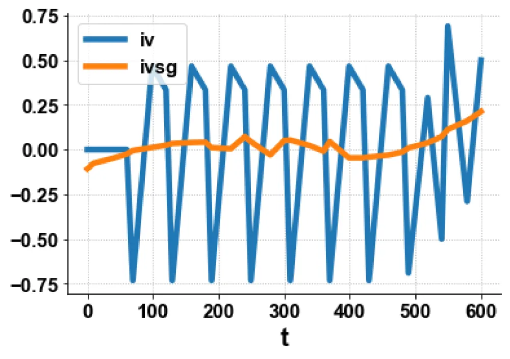
Figure 5a: MNLMPC iv, ivsg vs t.
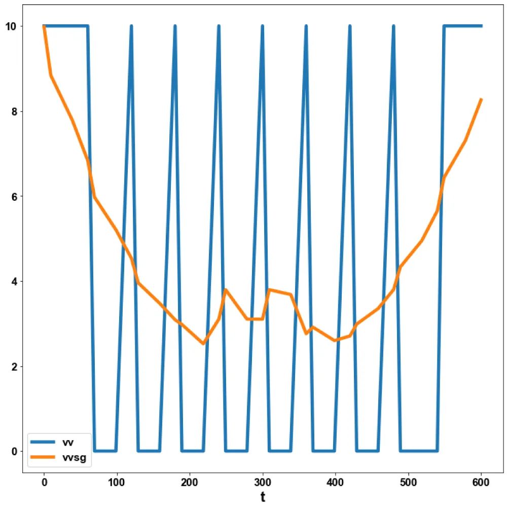
Figure 5b: MNLMPC vv, vvsg vs t.
Figure 5c: MNLMPC mv vs t.
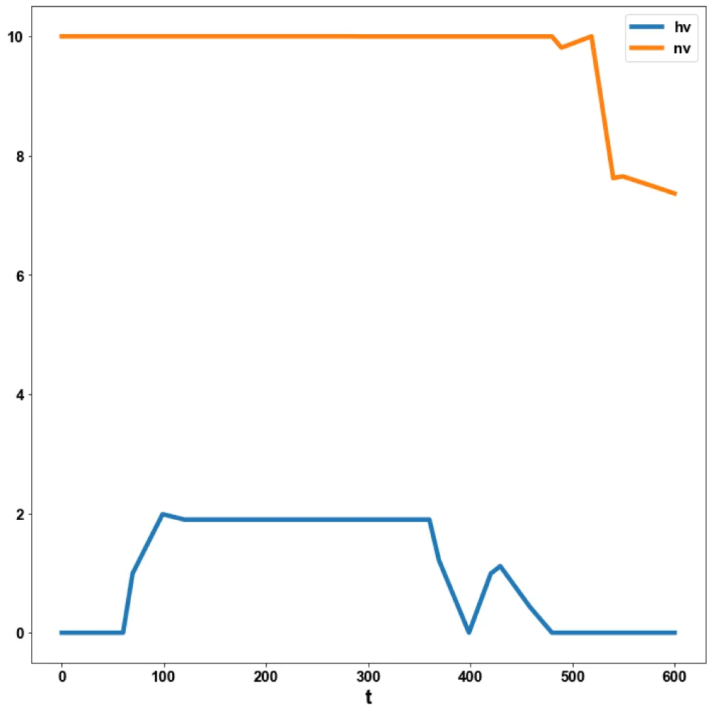
Figure 5d: MNLMPC hv, nv vs t.
The main conclusions of this work are:
Bifurcation analysis and multiobjective nonlinear control (MNLMPC) studies are conducted on the Hodgkin-Huxley model.
The bifurcation analysis revealed Hopf bifurcations and limit points.
Hopf bifurcation points, which cause unwanted limit cycles, are eliminated using an activation function based on the tanh function.
The Multiobjective nonlinear model predictive control calculations converge to the Utopia point (the best possible solution).
The limit points (which cause multiple steady-state solutions from a singular point) are very beneficial because they enable the Multiobjective nonlinear model predictive control calculations to converge to the Utopia point in the model.
This work is the first in open literature where bifurcation analysis and Multiobjective Nonlinear Model Predictive Control (MNLMPC) are integrated for the Hodgkin-Huxley model, and demonstrates how to avoid limit cycles in neurological problems and obtain the most beneficial control profiles.
Data availability statement
All data used is presented in the paper.
All the data can be reproduced. All the code developed can be reproduced.
Conflict of interest: The author, Dr Lakshmi N Sridhar, has no conflict of interest.
Dr Sridhar thanks Dr Carlos Ramirez for encouraging him to write single-author papers.
- Hodgkin AL, Huxley AF. A quantitative description of membrane current and its application to conduction and excitation in nerve. J Physiol. 1952;117(4):500–544. Available from: https://doi.org/10.1113/jphysiol.1952.sp004764
- Fitzhugh R. Mathematical models of excitation and propagation in nerve. In: Schwan HP, editor. Biological Engineer. New York (NY): McGraw-Hill; 1969.
- Chay TRL, Keizer J. Minimal model for membrane oscillations in the pancreatic β-cell. Biophys J. 1983;42(2):181–190. Available from: https://doi.org/10.1016/s0006-3495(83)84384-7
- Bedrov YA, Akoev GN, Dick OE. Partition of the Hodgkin-Huxley type model parameter space into the regions of qualitatively different solutions. Biol Cybern. 1992;66(5):413–418. Available from: https://doi.org/10.1007/bf00197721
- Guckenheimer J, Labouriau JS. Bifurcation of the Hodgkin and Huxley equations: a new twist. Bull Math Biol. 1993;55(5):937–952. Available from: https://doi.org/10.1016/S0092-8240(05)80197-1
- Bedrov YA, Dick OE, Nozdrachev AD, Akoev GN. Method for constructing the boundary of the bursting oscillations region in the neuron model. Biol Cybern. 2000;82(6):493–497. Available from: https://doi.org/10.1007/s004220050602
- Fukai H, Doi S, Nomura T, Sato S. Hopf bifurcations in multiple-parameter space of the Hodgkin-Huxley equations I. Global organization of bistable periodic solutions. Biol Cybern. 2000;82(3):215–222.
- Fukai H, Nomura T, Doi S, Sato S. Hopf bifurcations in multiple-parameter space of the Hodgkin-Huxley equations II. Singularity theoretic approach and highly degenerate bifurcations. Biol Cybern. 2000;82(3):223–229.Available from: https://doi.org/10.1007/s004220050022
- Zhu X, Wu Z. Equilibrium point bifurcation and singularity analysis of HH model with constraint. Abstr Appl Anal. 2014;2014:545236. Available from: https://doi.org/10.1155/2014/545236
- Dhooge A, Govaerts W, Kuznetsov AY. MATCONT: A Matlab package for numerical bifurcation analysis of ODEs. ACM Trans Math Softw. 2003;29(2):141–164
- Dhooge A, Govaerts W, Kuznetsov YA, Mestrom W, Riet AM. CL_MATCONT: A continuation toolbox in Matlab. 2004.
- Kuznetsov YA. Elements of applied bifurcation theory. New York (NY): Springer; 1998.
- Kuznetsov YA. Five lectures on numerical bifurcation analysis. Utrecht University; 2009.
- Govaerts WJF. Numerical methods for bifurcations of dynamical equilibria. Philadelphia (PA): SIAM; 2000.
- Dubey SR, Singh SK, Chaudhuri BB. Activation functions in deep learning: A comprehensive survey and benchmark. Neurocomputing. 2022;503:92–108. Available from: https://doi.org/10.1016/j.neucom.2022.06.111
- Kamalov AF, Nazir M, Safaraliev AK, Cherukuri, Zgheib R. Comparative analysis of activation functions in neural networks. In: 2021 28th IEEE Int Conf Electron Circuits Syst (ICECS); Dubai, United Arab Emirates. IEEE; 2021. p. 1–6. Available from: https://doi.org/10.1109/ICECS53924.2021.9665646
- Szandała T. Review and comparison of commonly used activation functions for deep neural networks. ArXiv. 2020. Available from: https://doi.org/10.1007/978-981-15-5495-7
- Sridhar LN. Bifurcation analysis and optimal control of the tumor macrophage interactions. Biomed J Sci Tech Res. 2023;53(5):MS.ID.008470. Available from: https://doi.org/10.26717/BJSTR.2023.53.008470
- Sridhar LN. Elimination of oscillation causing Hopf bifurcations in engineering problems. J Appl Math. 2024;2(4):1826. Available from: https://doi.org/10.59400/jam1826
- Flores-Tlacuahuac A, Morales P, Riveral Toledo M. Multiobjective nonlinear model predictive control of a class of chemical reactors. Ind Eng Chem Res. 2012;51(16):5891–5899.
- Hart WE, Laird CD, Watson JP, Woodruff DL, Hackebeil GA, Nicholson BL, et al. Pyomo – Optimization modeling in Python. 2nd ed. Vol. 67.
- Wächter A, Biegler LT. On the implementation of an interior-point filter line-search algorithm for large-scale nonlinear programming. Math Program. 2006;106:25–57. Available from: https://doi.org/10.1007/s10107-004-0559-y
- Tawarmalani M, Sahinidis NV. A polyhedral branch-and-cut approach to global optimization. Math Program. 2005;103(2):225–249.
- Sridhar LN. Coupling bifurcation analysis and multiobjective nonlinear model predictive control. Austin Chem Eng. 2024;10(3):1107.
- Upreti SR. Optimal control for chemical engineers. Boca Raton (FL): Taylor & Francis; 2013.
- Sridhar LN. Analysis and control of the bacterial meningitis disease model. Glob J Med Clin Case Rep. 2025;12(10):206–213. Available from: https://doi.org/10.17352/gjmccr.000227